Signals Agent

Project Summary

During the Proving Ground: Agentic Startup RAG-a-Thon, I built a prototype “signals agent” capable of analyzing noisy audio clips by performing multiscale FFTs, conducting spectral analysis, querying a web search API, and returning an explanation of frequency-domain events. You can think of it as an automated lab partner that listens, investigates, and explains what it hears.

Inputs:

• M4A/MP3 audio files (recorded live or pre-recorded)

• Core Pipeline:

  • audio2numpy → FFT → time + frequency binning → ReAct Agent (LlamaIndex) + Perplexity API → natural-language report

• Outputs:

  • CSV table of time-frequency energy

  • Richly annotated spectrogram (in terminal, colorized)

  • Conversational summary with web-sourced context and citations

By the end of the hackathon, the agent could detect and interpret dominant spectral peaks and trends, link them to plausible sources, and return results in under a minute — all running on local, commodity hardware.

Data Acquisition and Pre-processing

At the core of our signal analysis workflow is a flexible and adaptive approach to audio ingestion and segmentation. Before any meaningful interpretation can happen, the audio data must be properly captured, cleaned, and structured. This involves several key steps: loading the audio, converting formats, segmenting it across time and frequency, and allowing the agent to choose how to zoom in based on what it finds.

Loading the Audio

We support both pre-recorded audio (e.g., .mp3, .m4a) and live-recorded clips using a microphone. Regardless of the source, we standardize everything into WAV format and then convert it to a 1D NumPy array using audio2numpy and extract the sampling rate, which allows for easy manipulation in Python:

signal, sample_rate = open_audio("file.m4a")
# If audio is stereo, convert to mono
if signal.ndim == 2:
  signal = np.mean(signal, axis=1)

This mono conversion is important because spectral analysis assumes a single channel unless otherwise specified, and collapsing stereo to mono ensures uniformity during analysis.

Spectral Segmentation: Time and Frequency Bins

After loading, the signal is segmented across both time and frequency domains using a sliding window approach. We define a number of time_bins to divide the clip into equal-length windows (e.g., 10 bins for a 20-second clip = 2 seconds per slice), and we define freq_bins to segment the frequency domain into ranges (e.g., 0–100 Hz, 100–200 Hz, …, up to 2000 Hz).

# Setup bin edges
bin_edges = np.linspace(cutoff_lo, cutoff_hi, freq_bins + 1)
bin_labels = [f"{int(bin_edges[i])}-{int(bin_edges[i+1])}Hz" for i in range(freq_bins)]

Then, for each time slice, we compute an FFT and bin the energy:

fft_result = np.fft.fft(windowed_signal)
frequency = np.fft.fftfreq(len(windowed_signal), d=1/sample_rate)
power = np.abs(fft_result)**2

# Filter to within cutoff range
mask = (frequency >= cutoff_lo) & (frequency <= cutoff_hi)
frequency = frequency[mask]
power = power[mask]

# Bin the power spectrum
indices = np.digitize(frequency, bin_edges) - 1
binned_power = np.zeros(freq_bins)
for i in range(len(frequency)):
    if 0 <= indices[i] < freq_bins:
        binned_power[indices[i]] += power[i]

This generates a time-frequency matrix, where each row corresponds to a time slice, and each column corresponds to a frequency range. Each “square” of time and frequency contains a value that indicates the power density. This structured data is then either normalized (if freq_bins > 1) to show energy trends. Time bins help localize when something happens (e.g., a sudden burst of energy at 6.5 seconds). Frequency bins help identify what kind of signal it is (e.g., low-frequency mechanical hums vs high-frequency clicks).

Here is a video illustrating how adjusting frequency and time bins affects the information extracted from the spectrogram (Code for visual was done in JavaScript and can be found in my Signals Agent repo):

Spectral binning is a powerful tool. Smaller bins allow the agent to see finer resolution, isolating short-duration spikes or tightly grouped frequencies. Larger bins help identify broader trends and energy distributions. Adaptive binning allows the agent to first get a coarse overview and then drill into specific segments for further analysis. Rather than hardcoding ranges and bin sizes, we leave this decision to the agent. Based on what it observes in the broad scan, it can decide to zoom in:

Example agent instruction:

query = "Characterize the signals in the audio file located at ./data/audio3.mp3 by using the fft at 20 time bins and 20 frequency bins..."

Internally, the tool receives:

fft(file_path="./data/audio3.mp3", cutoff_lo=0, cutoff_hi=2000, time_bins=20, freq_bins=20)

If the agent sees interesting peaks in the 0–2000 Hz range between 8–10 seconds, it might issue a follow-up call with:

fft(file_path="./data/audio3.mp3", cutoff_lo=400, cutoff_hi=700, start_sec=8, end_sec=10, time_bins=5, freq_bins=10)

This recursive refinement mimics how a person might explore a spectrogram—start big, then zoom in where things look interesting.

This adaptive segmentation pipeline is essential for the agent’s success. By giving it control over resolution in both time and frequency, we enable a kind of multiscale thinking: a high-level scan followed by focused inspection. This not only makes the system more flexible, but also more intelligent—capable of narrowing down complex, noisy data to the most relevant features, just like an expert human would. In addition, this flexibility allows the agent to do whatever it thinks is best, creating some interesting out-of-the-box outcomes.

The Back End: The Agent & Its Tools

Now, let’s get into the meat of our system. At the core, we have an intelligent agent powered by the LlamaIndex ReAct framework. The agent’s job is to repeatedly reason about the audio it’s given: what sounds are present, where they occur in time, and what might be causing them. It doesn’t try to guess everything at once; instead, it searches, thinks, acts, observes, and repeats. Given a query (e.g., “Tell me what’s happening in this audio clip”), the agent starts with a broad FFT scan to get a general idea of the frequency activity across the full clip. Based on where energy spikes or trends appear, it drills down into specific time windows or narrower frequency bands. If a particular signal catches its attention, say, a strong 650 Hz tone between 8–10 seconds, it might use Perplexity to search for likely sources of that frequency. This decision-making is powered by a tool-based architecture. Tools are defined independently in functions.py, and the agent selects which ones to call, what parameters to use, and when to follow up.

Tool Registry

Below is a summary of the tools available to the agent:

The agent chooses among these tools dynamically, depending on its internal reasoning and user instructions. Let’s take a closer look at what each tool does and how it helps the agent accomplish its mission.

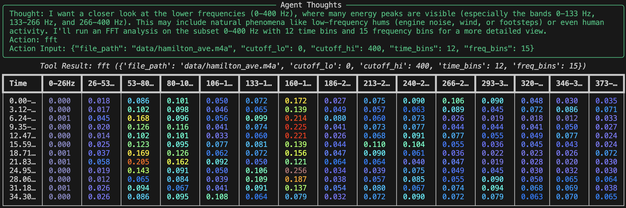
The FFT Tool

What is FFT? Prior to this project I was familiar with a Fourier Transform but not a Fast Fourier Transform, FFT (Fast Fourier Transform) is a mathematical algorithm that converts a time-domain signal (audio waveform) into its frequency-domain representation. In other words, it answers the question: “Which frequencies are present at any given time?” Real-world signals often overlap in time—multiple events happening simultaneously. FFT helps isolate what is happening when by breaking the signal into windows and computing a spectrum for each one. This creates a spectrogram, a 2D matrix of energy values: time vs. frequency.

The agent begins by calling the fft() tool with a wide frequency range and a modest number of time and frequency bins:

fft(file_path="data/audio3.mp3", cutoff_lo=0, cutoff_hi=2000, time_bins=20, freq_bins=20)

This returns a CSV-formatted spectrogram as a str:

Time,0-100Hz,100-200Hz,...,1900-2000Hz
0.0-1.0sec,0.01,0.03,...,0.00
1.0-2.0sec,0.00,0.05,...,0.01
...

This structured output allows the agent to spot peaks (high energy) and issue refined follow-ups like:

fft(file_path="data/audio3.mp3", cutoff_lo=600, cutoff_hi=700, start_sec=8, end_sec=10, time_bins=5, freq_bins=5)

That zoom-in behavior lets the agent focus on narrow, interesting regions just like a human would when inspecting a spectrogram by eye.

The Perplexity Tool

Once the agent identifies suspicious or dominant frequencies, it can ask: “What could be making this sound?”

This is where the search_perplexity() tool comes in. It connects to the Perplexity.ai API and lets the agent submit targeted queries like:

query = "Identify both man-made and natural sources of sound in the range of 600-700 Hz"

Perplexity returns a short, LLM-generated response with inline citations, helping the agent ground its answers in real-world knowledge. This is especially valuable for non-obvious signals (e.g., industrial hums, HVAC-systems, wind rustling tree leaves, etc.).

The Metadata Tool

Before diving into FFT, the agent often wants context: How long is this clip? What is its bitrate?

The file_meta_data() tool runs ffprobe under the hood to extract key metadata:

file_meta_data("data/audio3.mp3")

This returns:

Property,Value
Duration (seconds),10.23
Bit Rate (kbps),192000
Size (bytes),160000

This helps the agent plan how much to analyze and how to divide the signal over time. Even if the agent wasn’t prompted to run FFT analysis after, this information could still be valuable to the user.

The Record Audio Tool

The record_audio() tool allows live data capture during runtime:

record_audio(duration=10)

This uses pyaudio to stream audio from a microphone and saves it as a WAV file, enabling the agent to react to real-time input—not just preloaded data. In the future, I hope to incorporate an ambient running mode in line with this tool. I plan to have the agent start running its FFT analysis after recording a duration of audio after a certain threshold frequency is picked up or a significant shift in frequency range is received. By combining these tools, the agent becomes more than just a signal visualizer—it becomes a spectral reasoning system, capable of:

• Listening
• Investigating patterns
• Calling external knowledge
• Explaining what’s going on

All without any human intervention or hardcoded thresholds.

The Front End: User Interface and Output Formatting

While the intelligence of Signals Agent lives in its tools and reasoning loops, the way users interact with the system is still important. We designed a simple, elegant command-line interface (CLI) using Python’s rich library to guide users through the process, provide clear feedback, and display results in an engaging way. This front-end is implemented in two main modules: app.py and format.py.

The Audio Analysis Terminal

The app.py module is the user-facing entry point to the agent. When you run it, you’re greeted with an interactive terminal interface that guides you through every step—from selecting or recording audio to entering your analysis instructions. Here’s how the interaction works:

1. Welcome Screen: Users are greeted with a title screen and two options:

   • Use an existing file from the /data directory
   • Record new audio using a microphone

2. File Selection or Recording: If you choose to use an existing file, it displays a numbered list of .mp3 and .m4a files for selection. If you opt to record, it asks how long you’d like to record and streams microphone input to a WAV file.

selected_file = record_audio(duration=10)  # Records and saves as WAV

1. Analysis Instructions: You’re prompted to enter a natural-language task (e.g., “Analyze the humming sound and identify likely sources”). A default query is provided if you just hit Enter (it auto-fills).

2. Running the Agent: The app calls run_agent() asynchronously with your query and displays the agent’s thoughts, tool usage, and results in real time. This is helpful for seeing where the agent draws its information, and it allows the user to see the spectrogram at each resolution the agent chooses to analyze at.

3. Loop or Exit: Once the analysis is complete, it asks if you want to run another analysis or exit.

Spectrogram Visualization in the Terminal

Raw CSVs of frequency data aren’t easy to interpret on their own, especially in a terminal. That’s where format.py comes in. It converts the FFT tool’s CSV output into a colorized Rich Table, mimicking the look and feel of a spectrogram.

Key features of format_fft_output_as_rich_table():

• CSV Parsing: Reads the Time, Frequency Bin, and energy values from the CSV string returned by the FFT tool.

• Color Mapping: Maps each energy value to a hex color using the Jet colormap (matplotlib.cm.jet), where:

  • Blue = low energy
  • Yellow/Red = high energy

def _get_color_for_value(value, v_min, v_max):
  normalized = (value - v_min) / (v_max - v_min)
  r, g, b, _ = matplotlib.cm.jet(normalized)
  return f"#{int(r*255):02x}{int(g*255):02x}{int(b*255):02x}"

• Rich Table Output: Each time slice becomes a row. Each frequency bin becomes a column. The color-coding turns this into a kind of ASCII spectrogram, rendered right in your terminal window.

table.add_column("Time")
table.add_column("0–100Hz")
table.add_column("100–200Hz")
...

This feature is especially helpful for understanding how energy varies over time. The colorization makes important patterns—like pulses, peaks, or drops—visually obvious, even without switching to an external plotting tool, kind of like a heat map.

Why a Terminal UI?

Apart from the fact that we had limited time and wanted to focus on the subtsance of our project rather than a flashy shell, there were some technical reasons to keep it in the terminal. Not having a front-end reduces the total number of components involved in the process. This limits the number of connections where a fault or error could appear last minute. In a competition based event, this could be the difference between having something to present vs. not.

The terminal UI helps:

• Keep dependencies minimal
• Enable fast iteration and debugging
• Preserve compatibility with remote or low-resource systems
• Focus on substance over style while still delivering visual clarity through rich

That said, the architecture cleanly separates input/output from the core logic, so wrapping this in a GUI (or even a web interface) would be straightforward in the future which is something I definitely plan on doing.

Next Steps

While Signals Agent already performs multiscale acoustic analysis and intelligent reasoning over short clips, my vision goes further. There are two major directions I’m exploring: enabling ambient, real-time operation, and generalizing the agent to handle RF signals, not just sound.

Ambient Monitoring Mode

Currently, the agent operates in a request-response model, users manually provide audio, and the agent runs analysis on demand. A powerful next step is to enable a background monitoring mode, where the agent continuously listens to the environment and autonomously decides when to trigger deeper analysis. I’m planning to implement a threshold-activated recording system, where the agent passively listens through a microphone or sensors and continuously computes FFTs in short rolling windows (e.g., 1-second slices). Then, when spectral energy exceeds a configurable threshold or shows a sudden shift in frequency, it records a longer segment for a full analysis. For example, if a normally quiet environment suddenly produces burst of noise, or if a tone appears and begins to drift upward in frequency, the agent would recognize this as meaningful and capture a relevant time slice for interpretation. This transforms the agent from a reactive tool into a proactive observer, something more akin to a “watchdog” that only speaks up when something interesting is happening.

Expanding Beyond Audio: RF Signal Awareness

While our prototype is currently audio-focused, the architecture we’ve built, particularly the FFT engine, frequency binning strategy, and reasoning loop, translates cleanly to other signal domains, especially RF. RF signals, like acoustic ones, can be time-varying, noisy, and multicomponent. They require the same tools, FFT to analyze spectral content, time-frequency segmentation to capture dynamics, and contextual lookup to reason about unknown or unexpected signatures. By adapting the frontend to accept I/Q samples or raw RF captures from software-defined radios (SDRs), we could build a version of Signals Agent capable of detecting unauthorized transmissions in telecom networks, monitoring spectrum activity for electromagnetic interference, and identifying RF fingerprints of common devices in the environment. This opens the door to applications in communications monitoring, cybersecurity, defense, and wireless infrastructure diagnostics. The biggest lift will be handling different sample formats and extending the Perplexity tool’s prompting to cover RF domain knowledge—but the core reasoning framework is already in place.

Ultimately, the goal is to build an agent that can live ambiently in physical or electronic environments, continuously observe, and help people interpret invisible processes. Whether it’s a failing fan or a rogue RF emitter, I want the agent to listen, investigate, and explain.

Signal Agent’s Real World Applications

Predictive Maintenance in Factories

Imagine you have a “lights-out” factory line producing semiconductor wafers. In such a complex and precise industry as semiconductor manufaturing, the conditions of tools are even more important. Each wafer can be worth thousands of dollars, and the factory you’re running is so seamless, any delays or tool mishaps can set you back for weeks or even months. Machines and tools have a shelf-life, they wear down as you use them. These tools will often produce vibrations or shifts in frequency long before they break down. Signal Agent could potentially catch these, giving you a chance to order parts or new tools long in advance. If tuned enough, Signal Agent could even give e rough estimate of the time window in which the tool/machine breaks down. Our agent contributes the missing “why” layer: it doesn’t just raise an alarm; it explains that what the frequency anomaly could mean.

Smart Buildings & Environmental Monitoring

Beyond rotating machinery, many building systems emit distinctive acoustic signatures that shift subtly over time. One particularly valuable application is in HVAC (heating, ventilation, and air conditioning) systems. As air filters become clogged or fans degrade, these systems begin to operate less efficiently, often producing higher-frequency whines, lower throughput hums, or increased harmonic distortion in their acoustic profiles. By continuously monitoring ambient sound through ceiling-mounted microphones or embedded audio sensors, a spectral agent like ours could detect these shifts early—long before occupants notice discomfort or maintenance crews are alerted. For instance, a clogged air filter might manifest as a gradual rise in high-frequency energy as the system strains to maintain airflow. By visualizing these patterns in a live dashboard, building operators can trigger targeted interventions (e.g., replacing filters or tuning blower speeds).

Defense & Radio Frequency (RF) Signal Intelligence

Swap the microphone for a wideband RF front end and the same FFT-bin-explain loop can flag unauthorized transmitters, oscillator drift, or jamming attempts. This could be especially useful (and cool) since all of the remote-controlled devices like unmanned aerial vehicles (UAVs), ground vehicles like the MARCBOT, and even remote-controlled weapon systems all use RF. Because our agent queries the web, it can pull regulatory tables (e.g., FCC Part 15) and suggest compliance actions automatically.