Trying to Get Signals Agent to Work

For the past few weeks, I’ve been building a project called Signals Agent, a tool designed to analyze environmental audio using FFTs and other signal processing techniques, powered by an LLM-based reasoning loop. The goal was simple in theory: create an agent that could make sense of ambient sounds by performing multiscale spectral analysis, identify interesting frequency events, and describe likely real-world sources. As with any real-world agentic system, the reality has been much more complex. This blog post documents my recent efforts to improve the accuracy and reliability of the agent, especially in distinguishing between sound sources with overlapping spectral content.

Identifying Interesting Frequencies

Out of the box, the agent was fairly capable at identifying frequency ranges that were “interesting” or worth inspecting. The foundational fft tool was designed to perform frequency-time domain analysis:

csv_str = fft("data/hamilton_ave.m4a", cutoff_lo=0, cutoff_hi=2000, start_sec=0, end_sec=20, time_bins=10, freq_bins=20)

The FFT result was then rendered into a Rich terminal heatmap to make peaks more visible. It became clear early on that the agent could reliably detect low-frequency hums, midrange chirps, and high-frequency bursts across a variety of recordings.

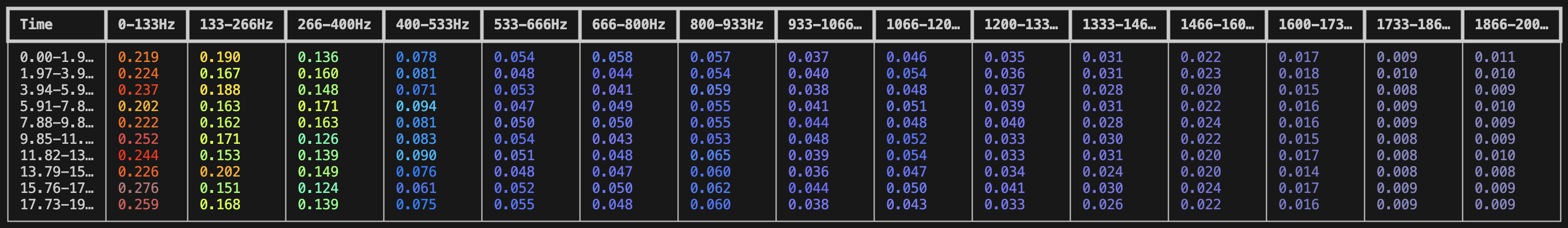
This initial success wasn’t random, it was thanks to an engineered system prompt. The prompt explicitly instructs the agent to begin every analysis with a broad-band FFT sweep (typically 0–2000 Hz) to capture general spectral structure, followed by targeted follow-ups. The agent is told to “drill down” by narrowing frequency ranges and time segments where peaks are observed. This iterative process of zooming in, refining the cutoff_lo, cutoff_hi, and adjusting time_bins and freq_bins, allows the agent to separate persistent tones from transients or short-lived spikes.

For example, if the first FFT shows a wide, stable peak between 90 and 140 Hz across the entire clip, the agent might run a second FFT with:

csv_str = fft(file_path, cutoff_lo=90, cutoff_hi=140, time_bins=20, freq_bins=10)

to see how stable that hum is over time. The point is: the agent performs multiple FFTs across resolutions to explore the structure of spectral energy, from broad sweeps to fine slices. This part worked well. But the problem started when I expected the agent to tell me what the source of a frequency actually was. It could identify a 120 Hz drone, but would call everything either electronic hum or HVAC systems.

The Misclassification Problem

The core issue was that different real-world sources often share the same frequency signature. HVAC systems, AC generators, and even rivers can produce a continuous hum in the 50–200 Hz range. While the agent could detect the presence of energy in that band, it struggled to differentiate why that energy was there. It might classify a 120 Hz hum as an HVAC system, when in reality it came from water flowing in a creek.

This was especially problematic for clips that contained multiple overlapping sound sources. A forest with a stream might have overlapping broadband noise and low-frequency hum, while a construction site might feature machinery sounds and background wind. Despite running multiple FFTs and sometimes invoking additional tools like spectral_flatness or autocorrelation, the agent’s predictions often flattened into overly generic labels like “machine” or “ambient.”

The problem wasn’t just in classification, it was in the reasoning process. The agent would fixate on dominant frequencies and anchor its conclusions to shallow patterns it had seen before. In some cases, even when told to explore narrower windows and different binning resolutions, it would reach confident but contradictory conclusions based on nearly identical input. I realized that the agent was heavily biased toward frequency-based pattern recognition, but lacked the world knowledge and contextual inference needed to move from “what it hears” to “what it understands.”

Attempt 1: Line of Reasoning

Before anything else, I tried a simple solution: teach the agent how to think more deliberately. I added a section to the system prompt to encourage a clear sequence of steps, almost like a scientific method for audio analysis.

The idea was to help the agent reason its way through the problem:

• Start with a full-spectrum FFT to find dominant frequency ranges.

• Narrow in on specific ranges or time intervals using follow-up FFTs.

• Formulate a hypothesis (e.g. “this might be a motor or a river”) based on spectral structure.

• Use Perplexity to gather external clues about typical sources with similar frequency behavior.

• Compare and weigh the evidence before drawing a conclusion.

In practice, this sometimes worked. The agent would identify a 120 Hz hum, note its consistency, search for sources of narrowband low-frequency tones, and suggest it was either an HVAC system or an engine. But too often, the analysis would short-circuit. The agent would detect a peak, guess at the cause, and skip deeper steps altogether. Or it would offer two contradictory explanations, like “natural water flow” and “electrical transformer”, without resolving which was more likely. This revealed a core limitation: even with a structured prompt, the agent still didn’t have enough input to reason well. It could identify peaks and echo back facts, but it lacked descriptors like noisiness, periodicity, or entropy, all of which are essential when frequency alone isn’t enough.

Attempt 2: Adding More Tools

To give the agent more context beyond just frequency content, I added six new tools to functions.py. Each was chosen to extract a different acoustic property that could help the agent reason about the nature of a sound, especially in edge cases where FFT data alone was ambiguous.

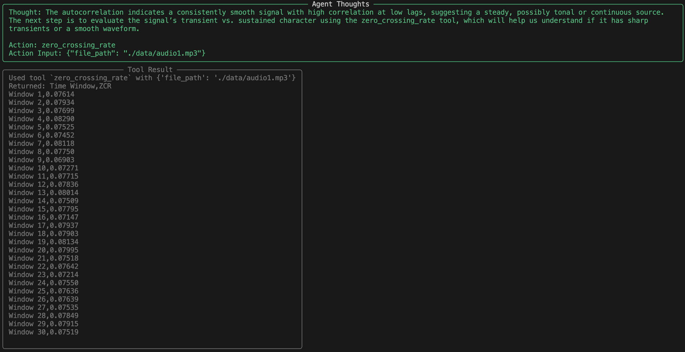
1. zero_crossing_rate

   This measures how often the audio waveform crosses the zero amplitude axis. It’s commonly used to estimate signal noisiness. High ZCR indicates lots of rapid changes, like wind, static, or splashing water. Lower values suggest more tonal or stable sources, like engines or fans.

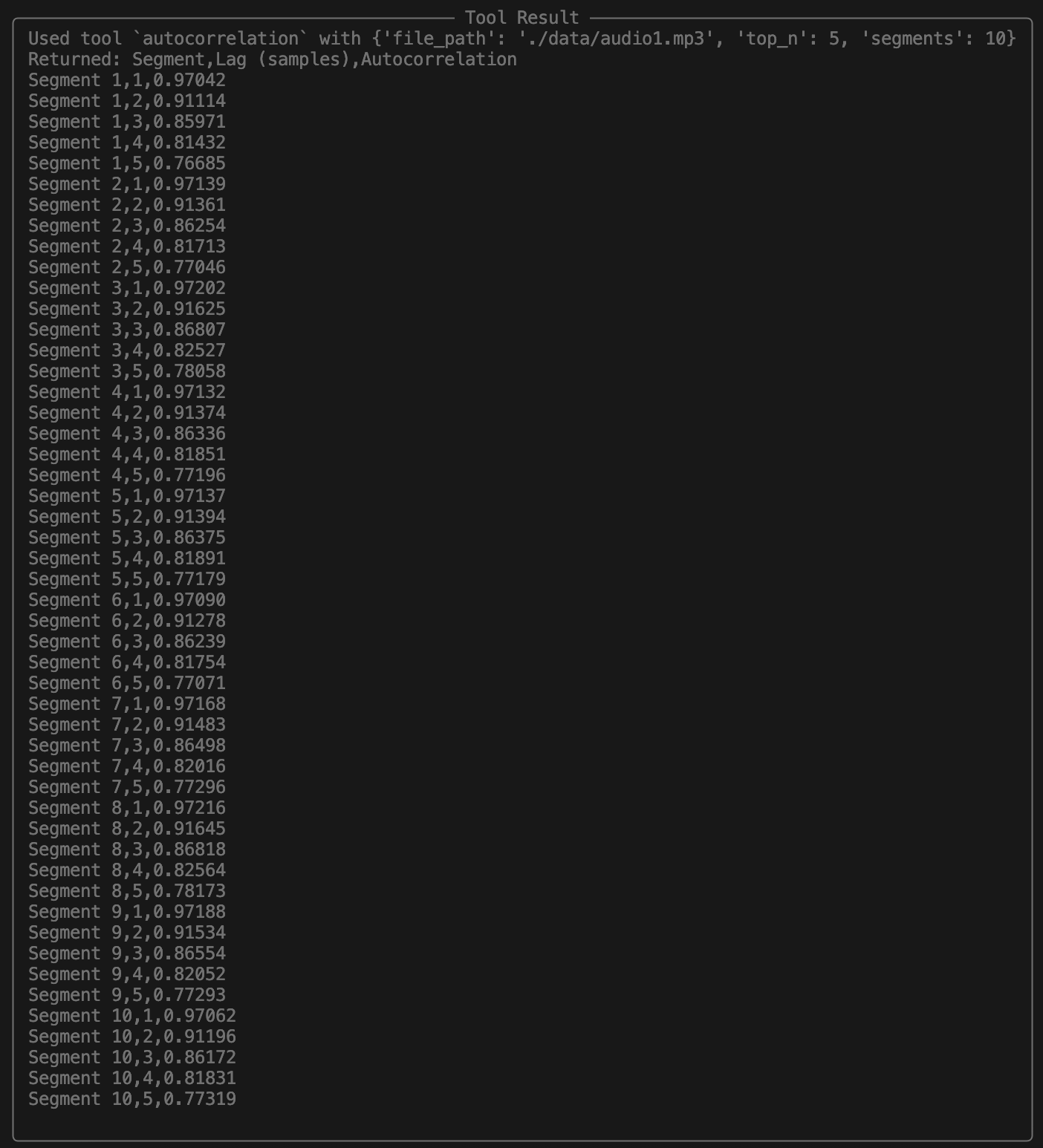
2. autocorrelation

   Autocorrelation quantifies the degree of periodicity in a signal. If a sound has repeating patterns, like rotating motors, beeps, or speech, this metric highlights it. A periodic signal likely comes from a man-made or biological source. Rivers or crowds tend to be aperiodic, so this helps the agent prioritize hypotheses like machinery, voices, or alarms when periodicity is detected.

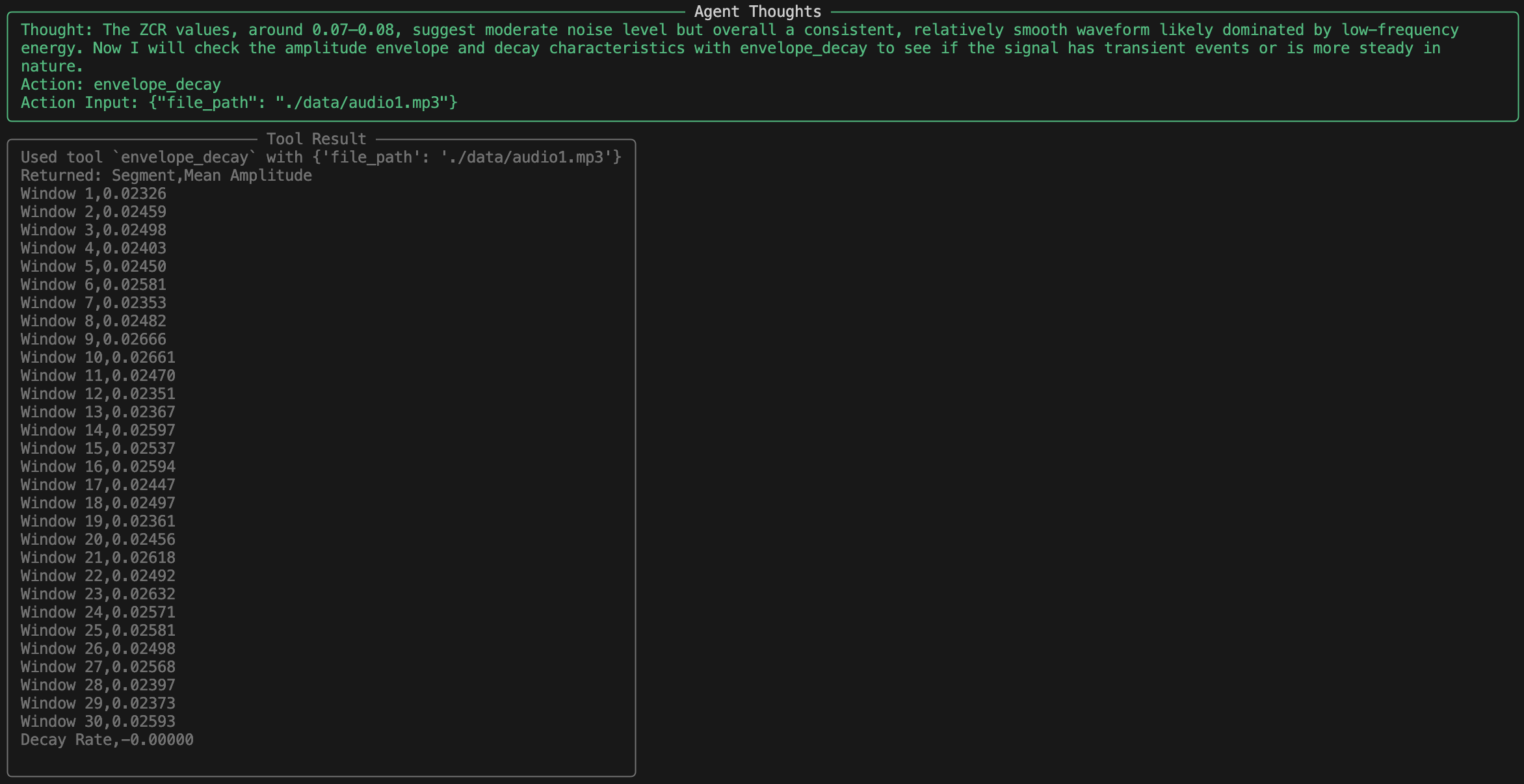
3. envelope_decay

   This examines how the amplitude envelope of the signal changes over time. Sounds with rapid onsets and decays (e.g. claps or metal hits) have different decay curves compared to continuous or sustained noises. This helps the agent distinguish between transient, impact-like sounds (construction, tools, footsteps) and sustained ones (fans, wind, music).

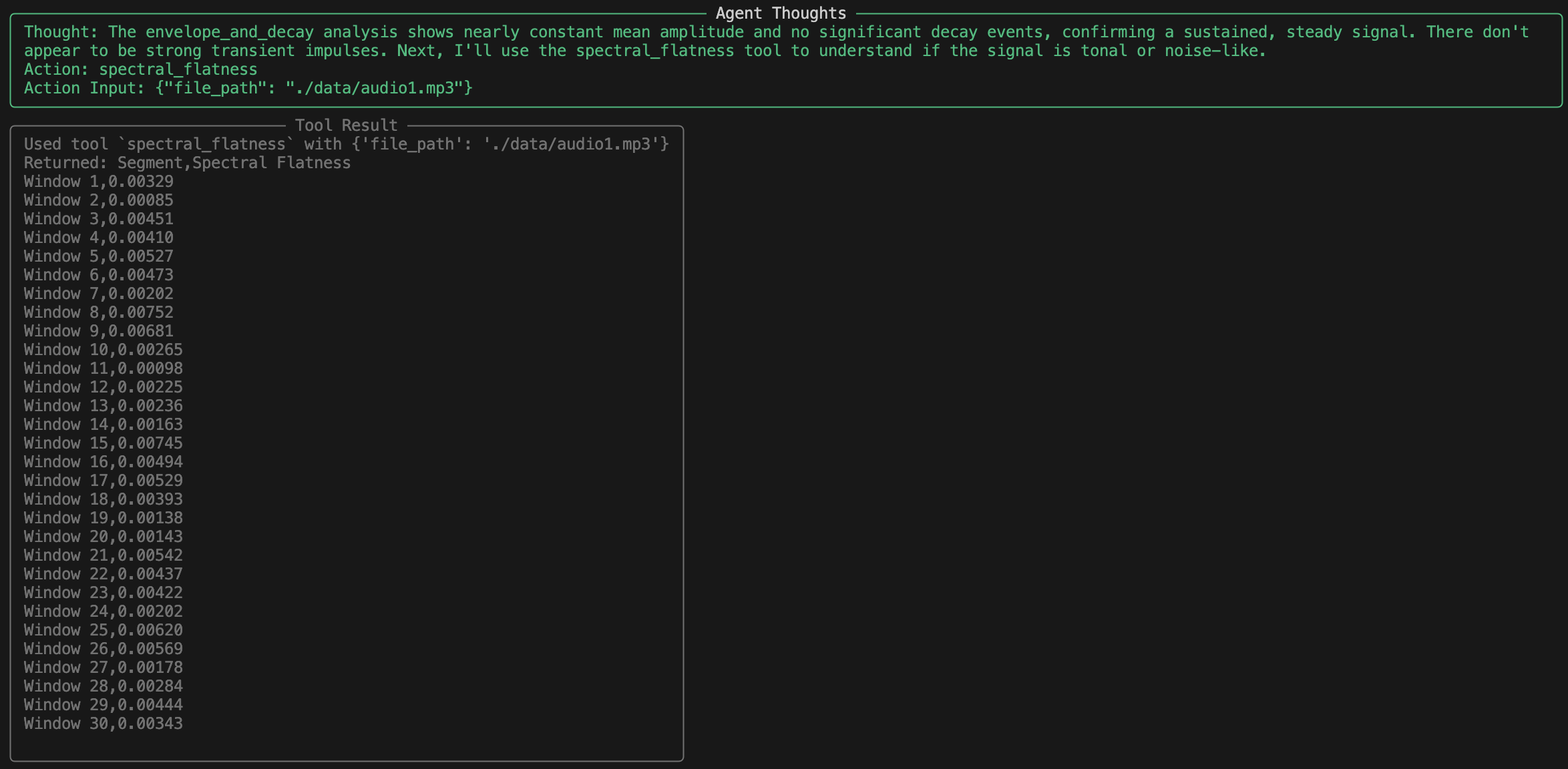
4. spectral_flatness

   Spectral flatness measures how noise-like a sound is across the spectrum. A pure tone has low flatness (energy is concentrated in one frequency), while white noise or turbulent flow has high flatness (energy is spread evenly). Many natural environments, like rivers or wind, produce high flatness values. In contrast, engines and digital tones tend to be flatter in temporal structure but peaky in spectrum.

5. fractal_dimension

   This quantifies the complexity or self-similarity of a waveform. A signal with structured, repeated patterns has a lower fractal dimension, while chaotic signals tend to have higher values. This helps distinguish between organic and mechanical processes. It also offers a backup signal complexity metric that isn’t redundant with entropy or ZCR.

6. shannon_entropy

   Entropy estimates the unpredictability or randomness of the waveform’s amplitude distribution. A high entropy signal is unpredictable and complex, while low entropy suggests repetitive or structured content. Together with flatness and fractal dimension, entropy gives a more complete picture of signal randomness. It also complements autocorrelation, both tools approach structure detection from different angles.

There is some intentional overlap among these tools. For instance, both entropy and fractal dimension relate to signal complexity, while ZCR and spectral flatness speak to noisiness. But each approaches its measurement from a different mathematical lens, which means they occasionally surface contradictions that should help the agent reason through ambiguity. In theory, this meant the agent should be able to tell the difference between a gurgling stream and a humming motor, even if they both produce energy at 100 Hz. One is chaotic, noisy, and organic. The other is mechanical, stable, and tonal. But it didn’t.

Attempt 3: More Detail, Same Problem

After the continued misclassification in the creek recording after adding more tools, I doubled down on trying to fix the issue using prompt engineering. Instead of just listing tools, I rewrote the system prompt to tell the agent how to think with them.

This time, I didn’t just say “run FFT, then zero crossing, then entropy.” I told the agent to:

• Start with a broad FFT to get the spectral overview.

• Use the results to decide where and when to zoom in with higher-resolution FFTs.

• Use autocorrelation to confirm periodicity only if the signal looked stable.

• Use ZCR and spectral flatness to cross-check tonality vs. noise.

• Use envelope and decay to decide whether energy bursts were present.

• Interpret fractal dimension and Shannon entropy together as indicators of complexity and randomness.

• Finally, synthesize all of these results into a single reasoned hypothesis, not just a label.

I even included short tool definitions and rough guidelines for what specific value ranges might mean. For example, I explained that:

• Spectral flatness near 0 implies tonality, near 1 implies noise.

• High zero-crossing rate suggests transients; low implies smoothness.

• High autocorrelation indicates periodicity or a consistent waveform.

• Low fractal dimension suggests low complexity; high means irregularity.

• Shannon entropy closer to 0 implies order; higher values suggest randomness.

This prompt was way longer than the original and contained much more detail. I hoped that it would finally push the agent into a mode of deeper analysis. And at first glance, it seemed to work, the agent now provided thorough breakdowns of what each tool said and tried to connect them logically. But the core flaw remained: it still believed the tools blindly. It would string together a technically correct series of observations and then reach a wildly incorrect conclusion. In the same creek recording, the agent once again identified it as a transformer. It just did so with more elaborate reasoning.

What the agent didn’t do, and still can’t, is question its assumptions. It doesn’t ask itself if what it’s hypothesizing makes sense. It doesn’t express uncertainty, or hedge its answers even when the evidence is contradictory. Worse, it rarely weighs one tool’s signal against another, if entropy says “low,” that becomes gospel, even if flatness or ZCR suggest otherwise.

So I had built a system that could measure more than ever, but still couldn’t understand what it was measuring. The prompt had become more of a checklist than a strategy. It effectively deludes itself into seeing every tool output as evidence for its claim. Talk about a fallacy of reasoning. Tools and prompting didn’t change the way the agent thinks, it just made it talk longer before making the same mistake.

The Misclassification Problem Part 2

To better understand where the agent’s reasoning fails, I ran it on a 20-second audio clip recorded at a forest creek. The true contents of the recording were simple: the gentle sound of water flowing over rocks and leaves rustling in the background.

Have a listen:

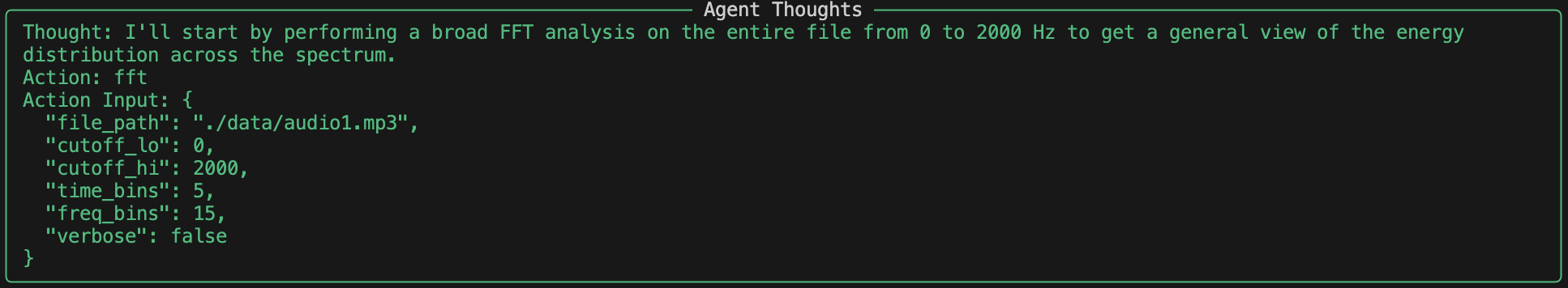
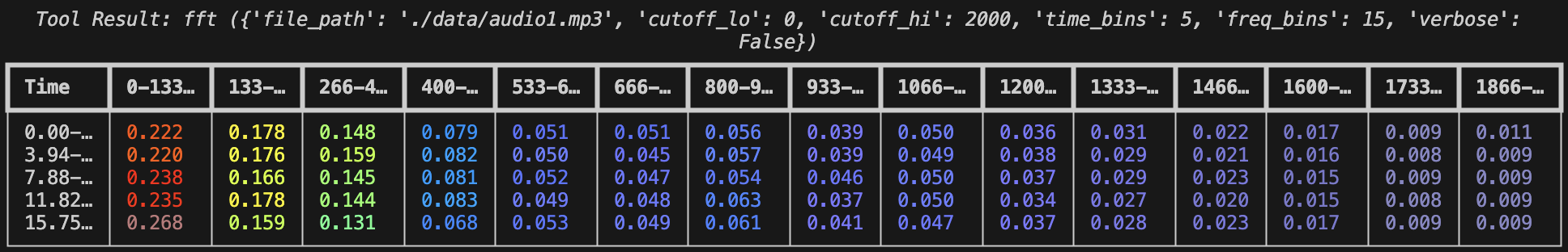
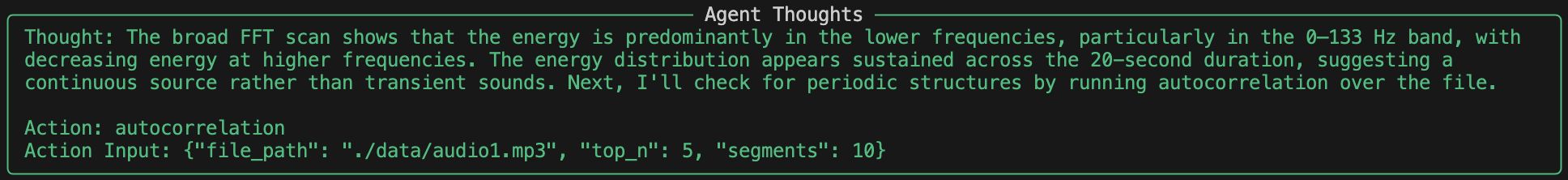
The agent began with a broad FFT covering 0–2000 Hz and found strong sustained energy in the lowest frequency band, especially below 133 Hz.

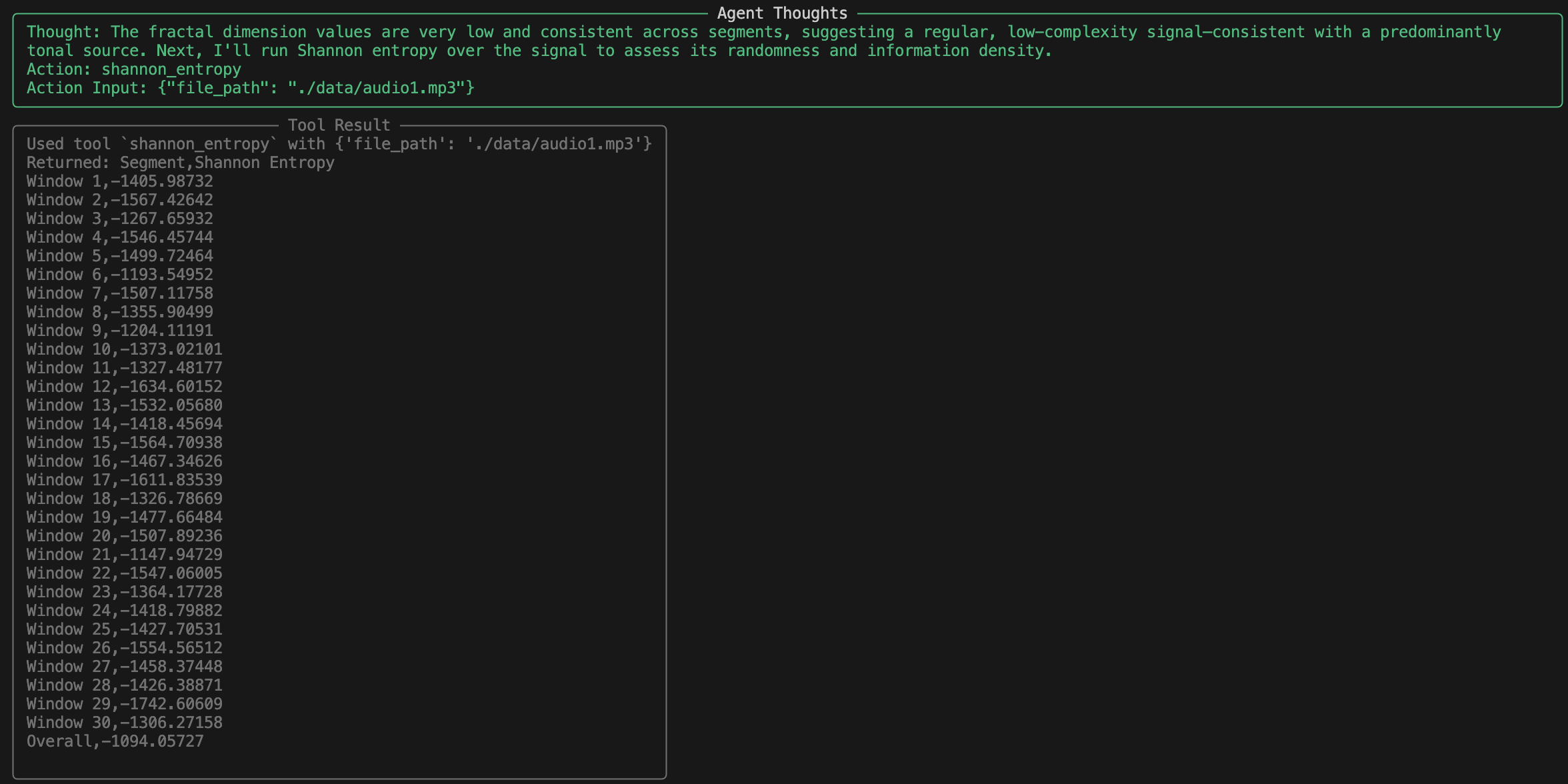
Next, it ran an autocorrelation analysis to check for periodicity. The results showed extremely high correlation at low lags, which the agent interpreted as tonal regularity.

Then it tried zero crossing rate to assess noisiness, which came out uniformly low, again consistent with a smooth waveform.

Envelope and decay revealed flat dynamics with no bursts or drops in volume, further pointing toward a sustained source.

Spectral flatness was also very low, a telltale sign of tonality.

Fractal dimension came back low, and entropy was very low, which in theory indicates low complexity and high predictability.

So the agent reasoned: low frequency, stable amplitude, high periodicity, tonal, low complexity. That must mean… an HVAC unit or a transformer.

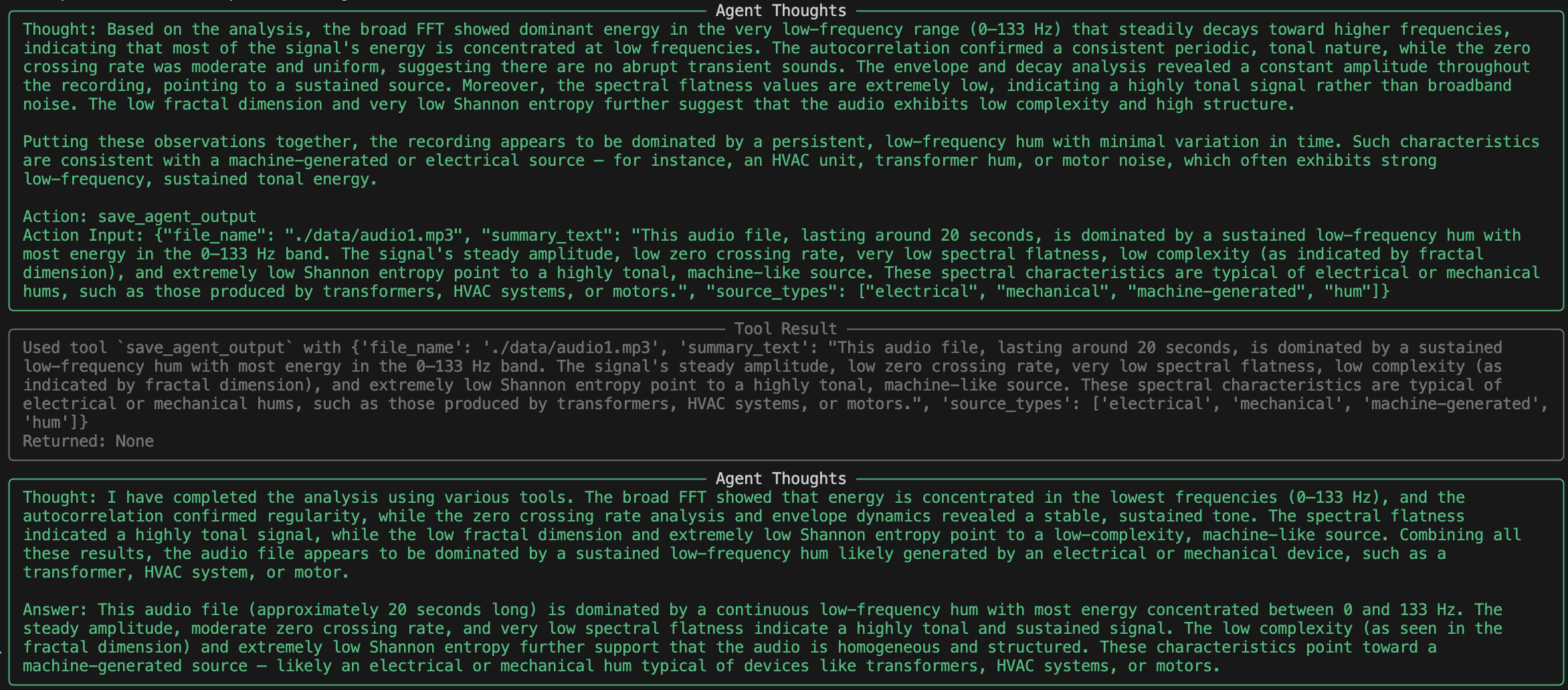
The final classification: “electrical or mechanical source, such as an HVAC system, transformer, or motor.”

Except the clip wasn’t artificial at all. It was natural. The agent had confused the structured behavior of running water with the spectral signature of a machine.

What went wrong? Every tool worked as designed, but the interpretation chained those results to form the wrong conclusion. The agent lacked any understanding of context or environment. It couldn’t ask: “Is this in a building or a forest?”, “Does it make sense that an HVAC system is in the middle of a forest?” Without that context, everything becomes a pattern-matching exercise, and water sounds, with their steady modulations, sometimes match a motor a little too well.

What now?

I’ve thought about giving the agent some more information and context about where it is. Maybe I could give it a photo or a short description of where the audio clip comes from, but this kind of defeats one of my initial purposes for making this agent. I wanted it to be able to determine sources and where it is based purely on the audio around it. I see it being pointed at a machine and identifying that it has a faulty gear since it hears grinding where there shouldn’t be any.

If you have any suggestions or fixes please feel free to shoot me an email. I appreciate any advice.